How To Show A Negative Percentage In Excel

23 aug, 2021

I currently have 2 cells in excel and im trying to find a formula to display the percentage. This is a time-honored way of formatting numbers as the sayings in the red and black Friday demonstrate.

Excel Negative Numbers In Red Or Another Colour Auditexcel Co Za

Select the cell or cells that may contain negative percentages.

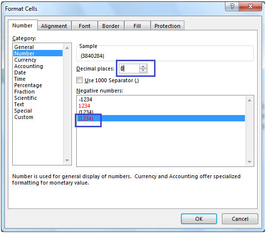
How to show a negative percentage in excel. Select the Number tab and from Category select Number. Is there any format in Excel 2002 that allows for it to be formatted. Click on Format Cells orPress Ctrl1 on the keyboard to open the Format Cells dialog box.

Add Brackets. Select the cell or cells that contain negative percentages. For the 8 decrease enter this excel percentage formula in b19.

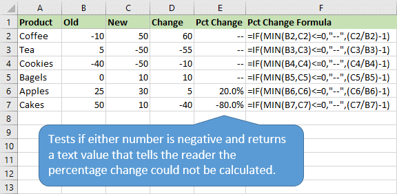
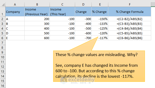
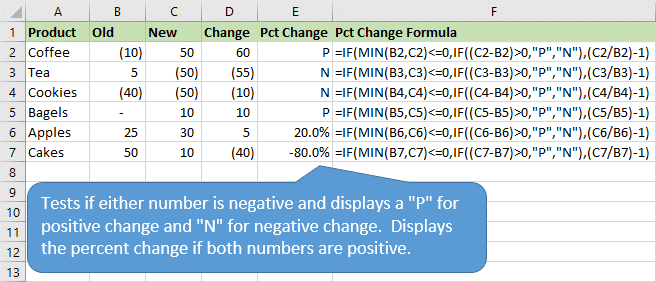
IFB10 C1 B1SIGNC1ABSC1B1 Examples B1before A1after. The greater the value change shows smaller percentage changes. Percentage change formula for negative numbersxlsx 198 kb.

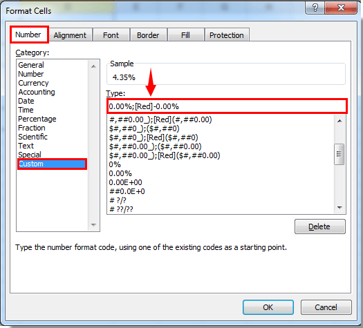
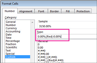
In the Format Cells box in the Category list click Custom. How do i change the axis of chart to percentage in excel 20132016. I have been able to format single cells to display negative percents Budget to Actual hours but I cannot copy the formatting to cells with positive percents without eliminating the format style I want.

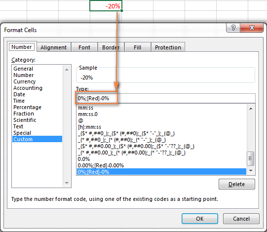
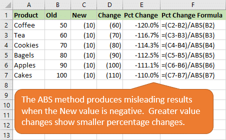
New value old value ABS old value This produces misleading results here the old value is negative and the new value is positive. Mark negative percentage in red by creating a custom format. If you want negative percentages to stand outfor example you want them to appear in redyou can create a custom number format Format Cells dialog box Number tab Custom category.

A common way is to mark negative variances to budget in red and positive in black. The percent change formula is used very often in excel. Learn how to calculate the percent change or difference between two.

IFB10 A1 SIGNA1-B1ABSA1-B1B1 To apply use percentage change to B1 D1 which should equal A1. It is good practice to make negative numbers easy to identify and if youre not content with this default Excel provides a few different options for formatting negative numbers. To display your negative numbers with parentheses we must create our own number format.

Microsoft Excel displays negative numbers with a leading minus sign by default. Open the dialog box Format Cells using the shortcut Ctrl 1 or by clicking on the last option of the Number Format dropdown list. Percent Change Formula In Excel Easy Excel Tutorial.

In the popping dialog choose one chart type you need the choose the axis labels two series values separately. But we must use that notion of change carefully. Add Parenthesis to Negative Percentages.

In the Format Cells dialog box you need to. The format should resemble the following. The fix is to leverage the ABS function to negate the negative benchmark value.

C4-B4ABS B4 The figure uses this formula in cell E4 illustrating the different results you get when using the standard percent variance formula and the improved percent variance formula. Select the cells right click on the mouse. In the Type box enter the following format.

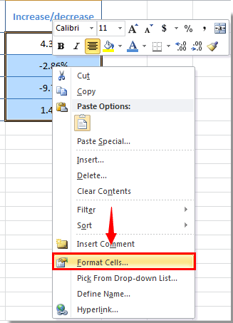
To select multiple cells hold down the Ctrl key as you. Right click the selected cells and select Format Cells in the right-clicking menu. One common way to calculate percentage change with negative numbers it to make the denominator in the formula positive.

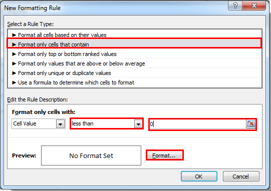
Percent Difference Formula Excel. On the Home tab click Format Format Cells. Choose Conditional Formatting from the Format menu.

The other way that you can display negative percentages in red is to use conditional formatting by following these steps. Want to express the percentage change as negative. Select the cells which have the negative percentage you want to mark in red.

Here is the formula that is commonly used. I need to display with the parenthesis 136for negative results but say 186 for positive results. A1 B1 C1 D1 should A1.

Add Brackets Minus Sign Mark Red All Negative PercentagesIn this Excel tutorial you ar. Or by clicking on this icon in the ribbon Code to. In the Negative Numbers box select the last option as highlighted.

Be sure to subscribe to the newsletter for more Excel tips and tricks. To compute percentage change C1. How to Mark Negative Percentage in Red in Microsoft ExcelIn this Excel tutorial you are about to learn two distinctive ways to mark or display negative per.

With the Positive Negative Bar Chart tool of Kutools for Excel which only needs 3 steps to deal with this job in Excel. Click Kutools Charts Positive Negative Bar Chart. When a formula returns a negative percentage the result is formatted as -49.

How To Make All Negative Numbers In Red In Excel